In this article, I’ll be explaining what gradient descent is in machine learning in a simple and easy to understand way.

What is Gradient Descent in Machine Learning?

Gradient descent is an optimization algorithm used in machine learning to predict data.

This is a probably really confusing explanation.

So, please keep reading so that we can understand the full picture.

An Example of Gradient Descent

Imagine that we’re trying to figure out a relationship between the average height of parents and the height of the child.

That is, if we know that the average height is, say, 68 inches, can we figure out how tall the child is?

Of course, the height of the child depends on a lot of factors, like their age.

A 6 year old child will be smaller than a 21 year old adult.

But let’s assume that they’re all 12 years old for now.

Resolving Linear Regression for Gradient Descent

We are trying to find the red line in the picture below.

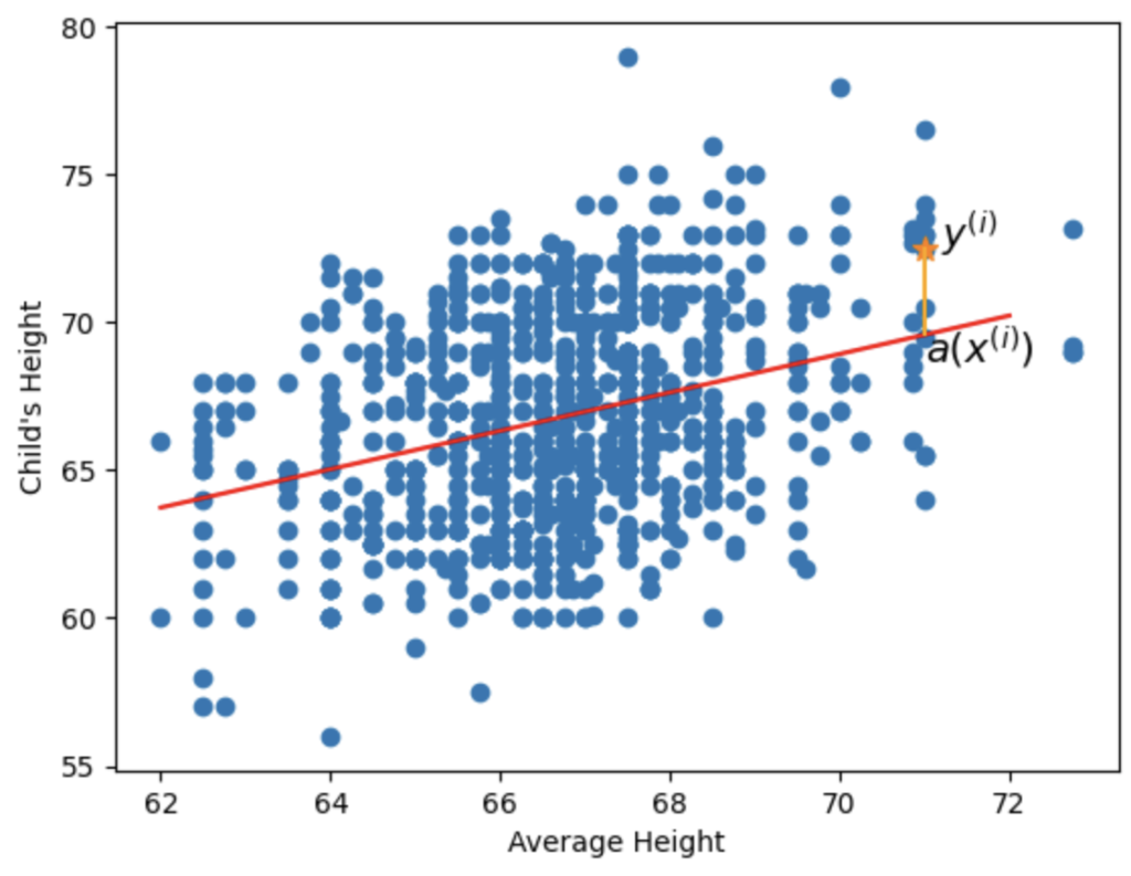
The red line will basically tell us “if the average height of the parents is 68 inches, then the child’s height is probably Y inches”

Remember linear equations from algebra?

You can represent any line with y=mx+b , where m is the slope, x is the x coordinate and b is the y-intercept.

In our case, we’re going to try to find a line, y_i = wx_i+b , where w is what we call the weight. The w is our slope, and b is our y-intercept.

And we’ve subscripted y with y_i and x with x_i to indicate that we’re now looking for the y that corresponds to the ith point.

So, basically, instead of looking for the entire line, the equation tells us that we’re just looking for the child’s height that corresponds to the average height x_i .

All we have to do is find the w and b .

Once we’ve found those two, we can just plug them into our formula: y_i = wx_i + b we’ll get the child’s height.

For example, if the weight is 1.1 and y-intercept is 8, then we can just say:

y_i = 1.1x_i+8 .

And if the average height of parent 1, x_i = 68 (which is about 5 foot 6), then we can say:

The height of child 1, y_1 is given by:

y_1 = 1.1*68+8=82.8 .

So, given that formula, the height of the child is 82.8 inches, which means that they’re 6 foot 9.

6 foot 9!?!?

Exactly. The weight w and y-intercept b in this example produced an unrealistic example.

So, how do we find a weight and y-intercept that will actually map the data correctly?

We use gradient descent.

The Sum of Squared Residuals

To begin with, let me introduce you to the sum of squared residuals.

The Error in One Point

Consider that the difference between the actual point y and the predicted point \hat{y} is equal to y_i – \hat{y_i} .

What this means is:

If our formula said that the height of child 1 was 82.8 inches and the actual height of child 1 was 70 inches, then:

y_1 = 70 hat{y_1} = 82.8

And the difference between the two is: \hat{y_1} – y_1 = 82.8-70=12.8

This means that our formula gave us an error of 12.8 inches for the 1st height of the child and the 1st height of the parent.

Great. So now, we know the error in our formula for the first point.

The Error in Every Point

But we want the error in every point.

This means that we have to take the sum of all of the errors, right?

SSR = \sum_{i=1}^{N}{(y_i – \hat{y_i})} .

This basically means “add up all of the errors from the first point i = 1 to the last point, i=N .”

If we had 3 points, then

SSR = \sum_{i=1}^{N}{(y_i – \hat{y_i})} .

= \sum_{i=1}^{3}{(y_i – \hat{y_i})} = (y_1 – \hat{y_1}) + (y_2 – \hat{y_2}) + (y_3 – \hat{y_3})

This is the same thing as saying “the error for the 3 points is the error in point 1 plus the error in point 2 plus the error in point 3.”

Squaring the Error

Great. Now, to prevent us from getting negative numbers and to make every error more drastic, we’re going to square everything.

Remember how previously, our error in point 1 was 12.8?

Guess what?

Now, it’s 12.8^2=163.84

And what if the error was 0.05?

Then, by squaring it, we’ll get 0.05^2=0.0025

Do you see the effect?

Squaring a big number gives a big number, while squaring a small number gives a smaller number.

And we’re using this for error, so if our error is really small and we square it, we’d be telling ourselves that the error is really small.

And if our error is really big and we square it, it would look like the error is really big.

And thus, we have our formula for the error, which we call the squared sum of least residuals.

SSR = \sum_{i=1}^{N}(y_i-\hat{y_i})^2

So this whole SSR monster is going to tell us how much error exists between our predictions and the actual data.

And remember our buddy \hat{y_i}, our prediction?

\hat{y_i} is actually equal to \hat{y_i}=wx_i+b, because \hat{y_i} is our prediction.

That’s the variable we’re trying to find the line for.

Thus,

SSR(w, b) = \sum_{i=1}^{N}(wx_i + b -\hat{y_i})^2

And SSR(w, b) is written in terms of w and b because w and b are both variables.

Minimizing the Error

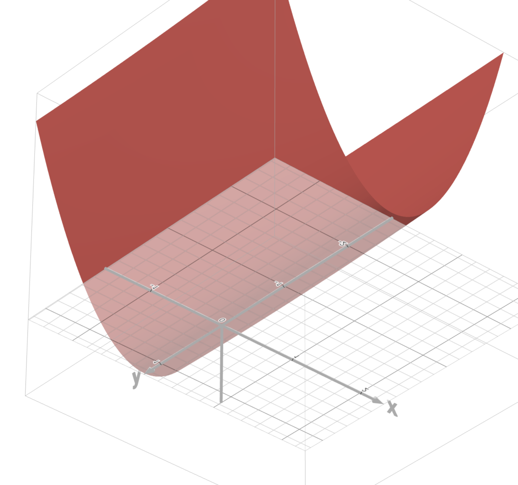
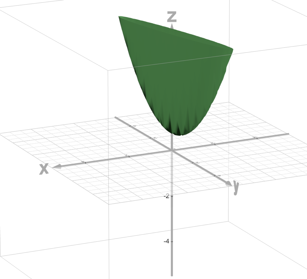
Now, we can model out error, SSR with a shape like this.

SSR(w, b) = \sum_{i=1}^{N}(wx_i + b -\hat{y_i})^2

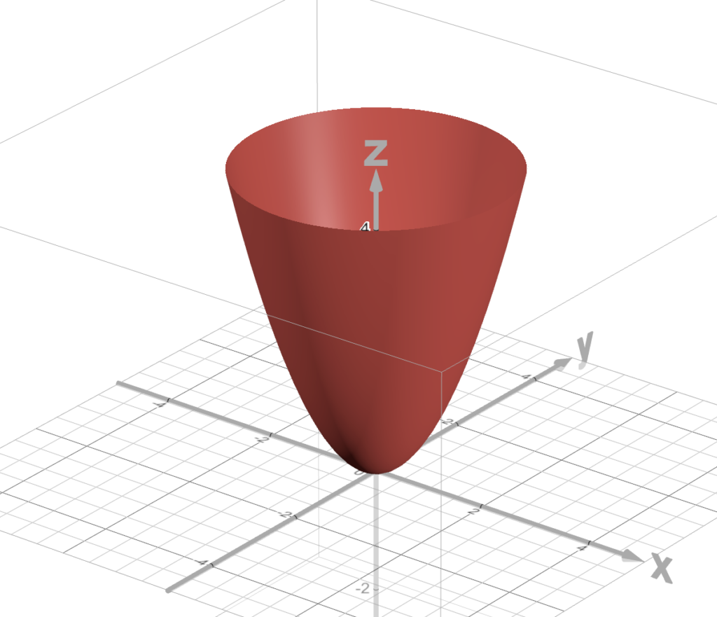
So, that red cloth looking thing is a model of our error.

Great.

It’s our error.

That means it’s bad.

So, we want this error to be as small as possible.

In other words, we want to minimize this error.

We want to figure out the points at the bottom of that red thing.

The bottom of that red thing (in this example) is that point at (0, 0, 0)

Now, note that the shape of this bowl looking thing varies.

Sometimes, it looks like a bowl.

Other times, it looks like, uhhh, whatever this thing is.

And we’re trying to minimize this error.

And one way of getting to the bottom of this error is by using gradient descent.

An Example of Gradient Descent

Let’s get started with an example of gradient descent.

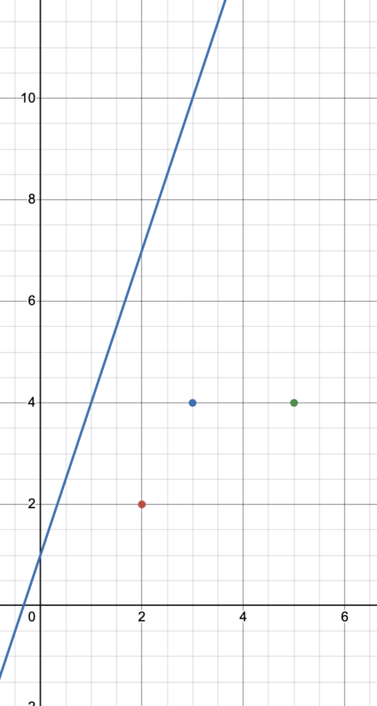
Let’s say that our points are these guys.

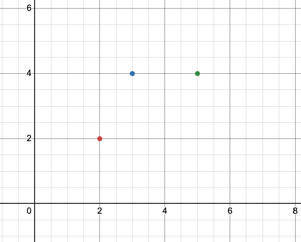
And we’re trying to find a line y=wx+b that minimizes the error, SSR .

SSR(w, b) = \sum_{i=1}^{N}(wx_i + b -\hat{y_i})^2

This is the same error equation from the previous section.

In gradient descent, we start out by picking a random value for w and b .

Let’s say that w = 3 and b = 1 .

Then, by substitution, our line becomes:

y = 3x+1

Take a look.

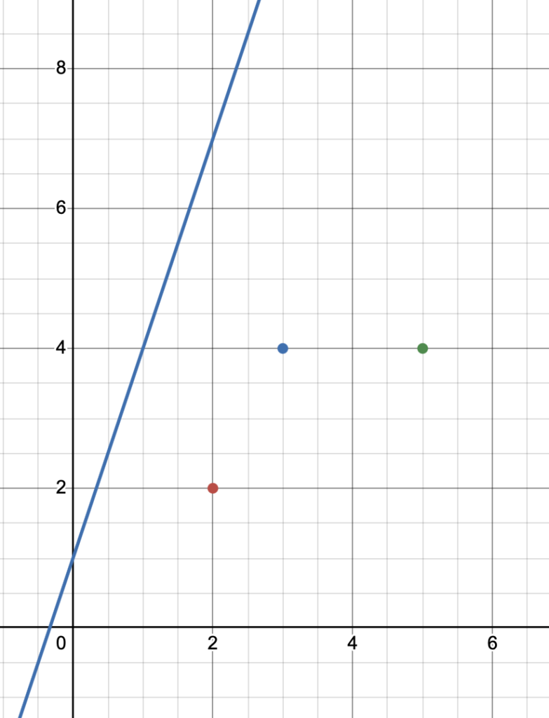
Our line, in blue, is super inaccurate, right?

It doesn’t go through any of the points at all. In fact, it’s pretty far away.

This means that our weight w and bias (y-intercept) b are inaccurate values.

We want to find a good w and b , so that our line has the least error.

This is where the gradient descent algorithm in machine learning comes into play.

Plotting the Error Function

SSR(w, b) = \sum_{i=1}^{N}(wx_i + b -\hat{y_i})^2

Now, we’re going to use gradient descent to model the minimization of this error.

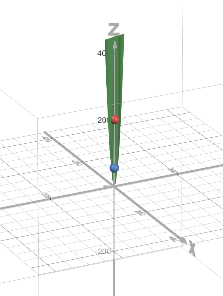
I’ve gone through and plotted every point and graphed it such that you can see the actual error graph.

This green flat bowl looking thingy is the actual error

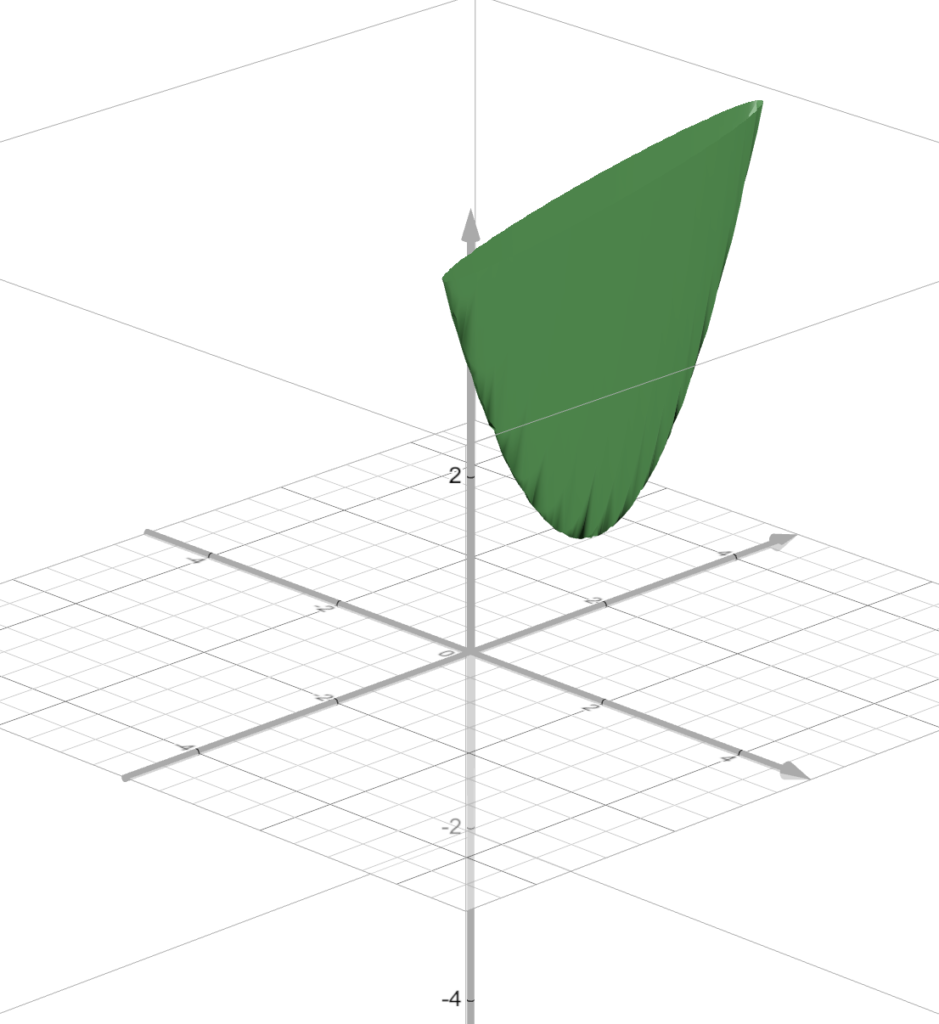
Hey, look!

From the top, it looks like a cucumber.

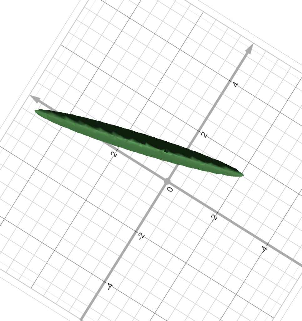
The x-axis (going left and right in the picture) is our “w” axis, representing our weights.

And the y-axis (going up and down in the picture) will be our “b” axis, representing the bias (y-intercept of the graph).

And we are trying to find the w and b that minimizes this error.

In other words, we’re trying to find the w and b that takes us to the bottom of this vegetable looking thing.

And one way to do this is by using the gradient descent algorithm.

Finding the Gradients of the SSR

The gradient descent algorithm starts by choosing a random “w” and “b”, as we did earlier to get this line:

Here, w = 3 and b = 1, giving us y=3x+1

SSR(w, b) = \sum_{i=1}^{N}(wx_i + b -\hat{y_i})^2

And in our SSR error function (the vegetable graph), that point is represented by that gray ball, at the point 205.

This means that SSR(3, 1) = 205 .

That 205 is our error.

That’s basically how bad our line is at predicting the points.

It’s 205 bad. OK!

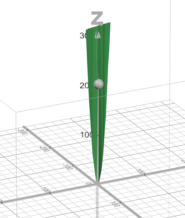
Remember, we want to find the w and b that take us to the bottom of that curve because at the bottom of that curve, our error will be very small.

To do this, imagine that you’re standing on that point.

There’s one direction that is the steepest direction. That is the gradient.

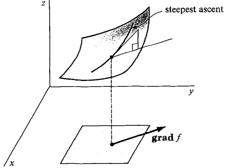
In the picture above, you can see that the gradient, grad f , points at the steepest direction.

The gradient, since it is the steepest direction, it is the direction at which will be the hardest to climb.

But, we’re trying to go down, aren’t we?

So.. instead of trying to go up in the steepest direction, why don’t we go down in the steepest direction? That means that we’ll go down in the direction that will get us to the bottom the fastest.

Thus, we have our gradients.

\nabla SSR =\begin{bmatrix} \displaystyle\frac{\partial SSR}{\partial w} \\ \displaystyle\frac{\partial SSR}{\partial b} \end{bmatrix}

Remember that \nabla SSR will get us in the steepest direction.

We want to go down to find the minimum of the SSR, not up.

So, to get to the minimum of the error, why don’t we just subtract w and b by the gradient.

If we subtract the gradient, then we’ll be decreasing w and b by the steepest direction.

And if we keep on subtracting this gradient over and over again, eventually, we’ll reach the bottom and we’ll get the w and b needed to minimize the error!

w_{new} = w_{old} – \frac{\partial SSR}{\partial w_{old}} b_{new} = b_{old} – \frac{\partial SSR}{\partial b_{old}}

I won’t be getting too deep into the multivariable calculus in this thread, but here is the gradient of SSR:

\nabla SSR =\begin{bmatrix} \frac{\partial SSR}{\partial w} \\ \frac{\partial SSR}{\partial b} \end{bmatrix} = \displaystyle\begin{bmatrix}\displaystyle\sum_{i=1}^{N} 2 x_i (w x_i + b -\hat{y_i}) \\ \displaystyle\sum_{i=1}^{N} 2 (w x_i + b – \hat{y_i})\end{bmatrix}

And, we’re going to introduce a new variable \alpha , which we’re going to call the learning rate.

And our \alpha will be between 0 and 1 .

Using the Gradient Descent Algorithm

So, we have:

w_{new} = w_{old} – \alpha \frac{\partial SSR}{\partial w_{old}} b_{new} = b_{old} – \alpha \frac{\partial SSR}{\partial b_{old}} \nabla SSR =\begin{bmatrix} \frac{\partial SSR}{\partial w} \\ \frac{\partial SSR}{\partial b} \end{bmatrix} = \displaystyle\begin{bmatrix}\displaystyle\sum_{i=1}^{N} 2 x_i (w x_i + b -\hat{y_i}) \\ \displaystyle\sum_{i=1}^{N} 2 (w x_i + b – \hat{y_i})\end{bmatrix}

Now, if we were to run these equations one time (we call this one epoch), with \alpha = 0.005 we would get:

w_{new} = 3 – 0.005 \displaystyle\sum_{i=1}^{N} 2 x_i (w x_i + b -\hat{y_i}) = 2.12 b_{new} = 1 – 0.005 \displaystyle\sum_{i=1}^{N} 2 (w x_i + b – \hat{y_i}) = 0.17

And now, we have new values for w and b!

If we plug in these values for our SSR:

SSR(w, b) = \sum_{i=1}^{N}(wx_i + b -\hat{y_i})^2 SSR(2.12, 0.17) = \sum_{i=1}^{N}(2.12x_i + 0.17 -\hat{y_i})^2 = 58.0419

Our error, with w = 2.12 and b = 0.17 is now only 58.0419.

And in the picture below, it’s represented by that blue dot.

Look at how much we’ve improved!

Our error is a lot less.. and if we look at our line, using the new values for w and b…

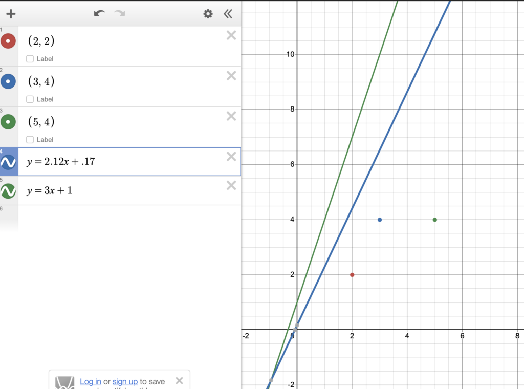
The blue line is our new line, which is a lot better than the green line!

Now, imagine if we ran the same algorithm again, (another epoch), and again, and again, …

w_{new} = w_{old} – \alpha \frac{\partial SSR}{\partial w_{old}} b_{new} = b_{old} – \alpha \frac{\partial SSR}{\partial b_{old}} \nabla SSR =\begin{bmatrix} \frac{\partial SSR}{\partial w} \\ \frac{\partial SSR}{\partial b} \end{bmatrix} = \displaystyle\begin{bmatrix}\displaystyle\sum_{i=1}^{N} 2 x_i (w x_i + b -\hat{y_i}) \\ \displaystyle\sum_{i=1}^{N} 2 (w x_i + b – \hat{y_i})\end{bmatrix}

The results get better and better.

Note that in this example, I used a large learning rate to demonstrate the effects of gradient descent.

In practice, we’d use an even smaller learning rate.

Conclusion

And there you have it!

To conclude, gradient descent is an algorithm that we use in machine learning to find the “best fit line” across a bunch of points.

Here are the graphs I created:

3D graph: https://www.desmos.com/3D/p1lrfiqlii

2D graph: https://www.desmos.com/calculator/vnzyq8t1kn

Thanks for reading!